Notes on DDPMs (Diffusion Denoising Probablistic Models) -- what is it and how the math works

Journey into Diffusion Models Part 1: What is Diffusion? Building the Math Intuition

Preface:

This delayed post has been planned under consideration for a while, and I’m writing it as a way of sharing interesting insights as well as journaling down my learning curve. I know there are plenty of articles out there on the same subjects, and I am sure they all do a great job explainin in different approaches (in fact, I spent quite some time reading and synthesizing a handful of them, of which I have attached in the source). Though, if you are interested in an easily understood version from an undergrad’s point of view, this is would be your go-to.

Diffusion models —Introduction:

You must have heard about Stable Diffusion, Mid Journey, DALL-E or other text to image models that create images with prompts, which all have diffusion models operating under the hood and are categorized as generative models. Diffusion models are like LLMs (if you are familiar with products like ChatGPT) are trained on existing image inputs as training data, and after pretraining, can generate new images mimicing the images they are trained on.

Historically, images are first generated by GAN — Generative Adversarial Networks since thier invention in 2014. On a high level GANs operate in an adversarial way by training a generator that is responsible of generating images, and a discriminator that evaluates whether the input image is generated by the generator, or real data from sample images. These two components play a minimax game where one tries to generate fake images as realistic as possible, and the other also getting better at identifying whether the images are real or fake. During training the discriminator gives feedback of the evaluation result to the generator through backpropagation, improving the quality of the next generated imags. The generator “learns” by time how it can generate forged images closer to the realistic ones.

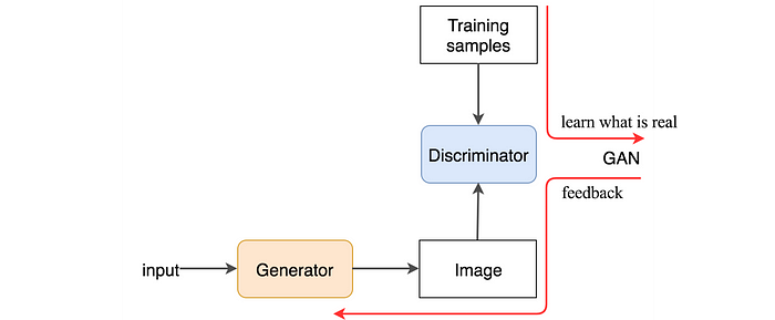
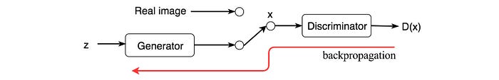
source: What is GAN? Medium article GAN architecture

However, GAN has its disadvantages despite its speed at inference, its down sides lies in training where the model might experience collapse due to issues like the vanishing gradient problem. As a result a limited diversity of images, or even worse, only one image is generated as the discriminator gets strong too quickly, and the generator only finds its way through a few examples that goes undetected by the discriminator. Therefore, with diffusion models which produce stable and high quality results, GAN’s disadvantages in image generation is out performed; although in contrast, diffusion models are slower as they take an iterative approach when generating one image vs. GANs do a single forward pass.

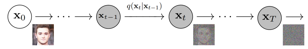
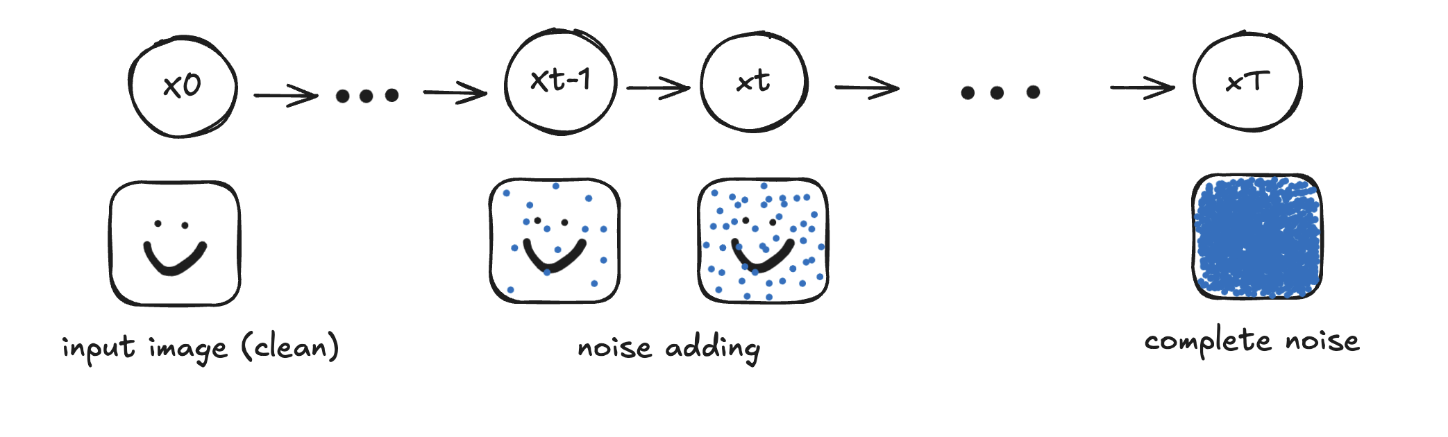
Essentially, diffusion models are build upon the basis of Markov chains. The time element comes from their training and inference. Their training process consists of injecting clean images, continuously adding Gaussian noise little by little until the whole image is covered by pure noise, meanwhile with the forward process (the process of adding noise), a neural network learns from the reverse (denoising) process, and perform denoising iteratively to generate a image at inference time. Thus, from a very high level point of view, the Markov element comes from “the current state of noise dependes on the previous noise state”. Don’t worry if you do not yet have an intuition of what’s going on, we will be discussing and formally define these terms more in detail progressively down the post. Now there are some major models within the family, and today we will be looking at DDPMs (Diffusion Denoising Probablistic Models), which takes the process mentioned above. Though we will be focusing more on the theoretical maths in this post, we will be dicussing more in depth the architecture — U-Net strucutrue in the next posts.

Forward Process: Noising

There are 3 main components to understand in DDPMs:
- the forward process (noising or diffusion process)
- the reverse process (denoising or reverse diffusion process)
- training objective & loss

The forward process (also called the diffusion process) is a Markov chain that slowly adds Gaussian noise (noising) to data, in this case image data over T timesteps at which the image becomes “pure Gaussian noise” (isotropic Gaussian noise). At each step, it adds some pre-determined amount of noise decided by the hyper parameter 𝛽t (a small positive number between βt∈(0,1) ) to the data.
The initial sate x0, where q is the true data distribution:

Data point x0 sampled from real Gaussian distribution q(x).

Single step noise addition: So to get from previous state xt-1 to a slightly noisier state xt, xt is sampled as: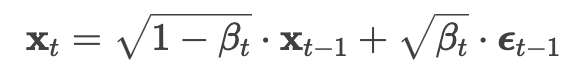

Noise schedule βt or αt how fast the signal x0 is currupted, they control how fast and slow the two variables decay.
- signal scaling: √αt –> 0 (x0 signal decays)
- noise scaling: √1-αt –> 1 (noise ϵ dominates)
In probability representation: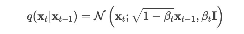

• The new state xt is constructed given the previous state xt-1. The Gaussian mean is: (latex)${text} and variance is: (latex)${text}
• 𝛽t I means we are in a multidimensional scenario, I is the identity matrix, meaning each dimension has the same standard deviation 𝛽t.
  

Full forward process: The entire noising process from xo to xT can be factorized by this: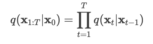

The symbol x1:T means applying q repeatedly from timestep 1 to T, or can be represented alternatively by x1,x2,…,xT.

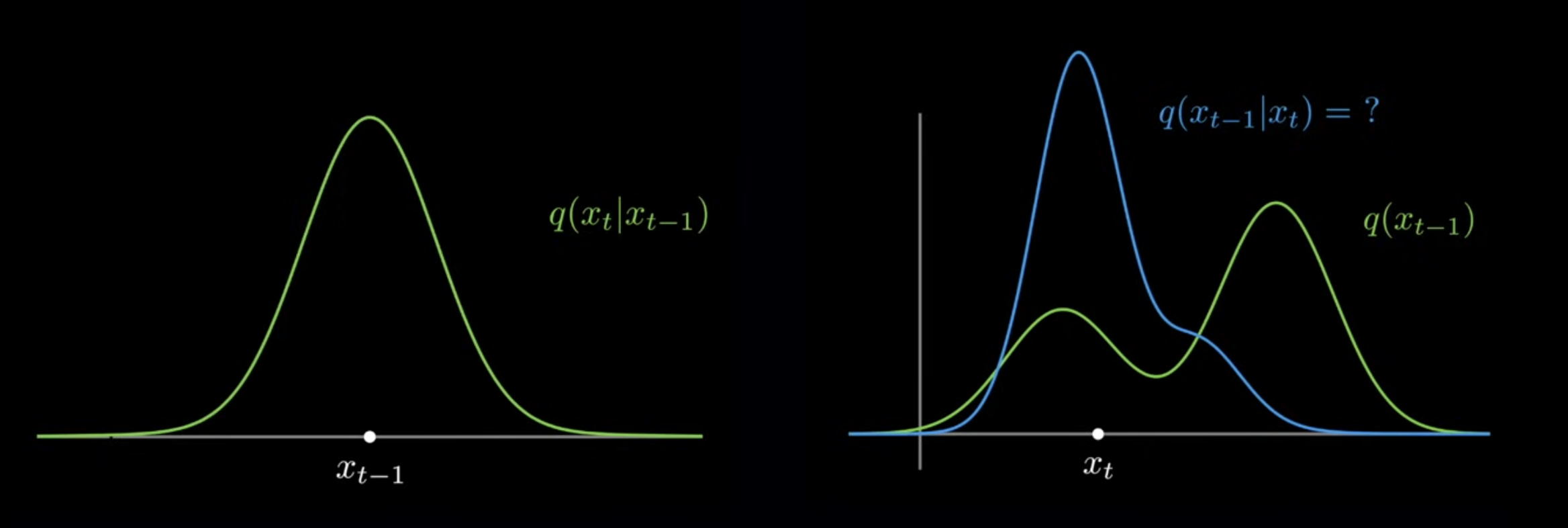
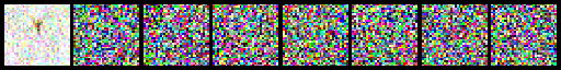
Now we can bring back the reason why βt being very small is useful. From the equation above the variance of the normal distribution noise is sampled from depends on βt, intuitively during the reverse process when the amount of noise to reduce is predicted from the distribution, a smaller variance from the prior distribution q(xt-1|xt) enables the model to predict xt from a “narrower” distribution. Below are graphs that help you visualise the concept ( this video does a greate job building up the intuition).

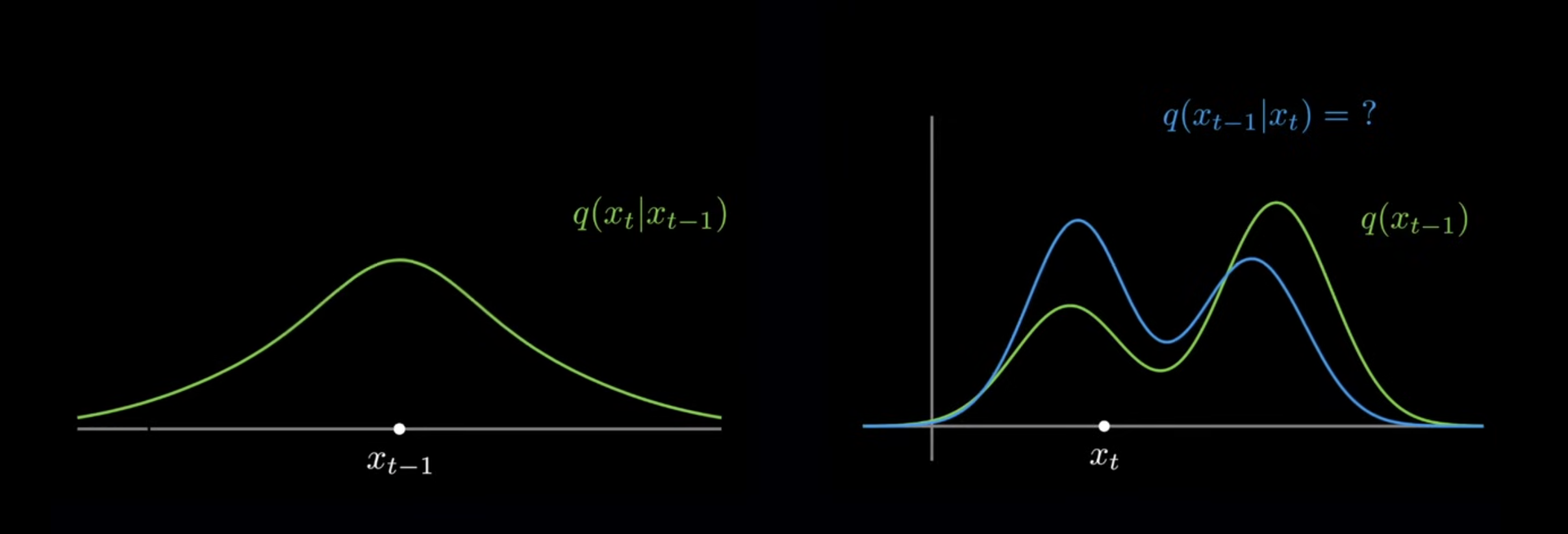With a smaller βt, the prior distribution variance is smaller: In fact, βt can be either fixed or a schedule st. β1< β2 < .. < βT, βt∈(0,1). Different Beta schedules (AKA variance schedule) result in different effects. Below are some examples to explain the effect of different βt schedule on the forward process:

noise_scheduler = DDPMScheduler(num_train_timesteps=1000)

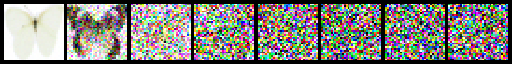
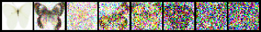
One with too little noise added:

noise_scheduler = DDPMScheduler(num_train_timesteps=1000, beta_start=0.001, beta_end=0.004)

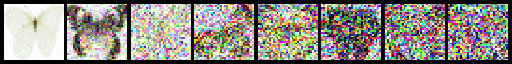
One with too much noise added:

noise_scheduler = DDPMScheduler(num_train_timesteps=1000, beta_start=0.1, beta_end=0.004)

The ‘cosine’ schedule, which may be better for small image sizes:

noise_scheduler = DDPMScheduler(num_train_timesteps=1000, beta_schedule='squaredcos_cap_v2')

Reverse Process: Denoising

The reverse process is another Markov chain that starts from xT — an image with complete noise, back to x0 a clean image. During the process the model learns how to do the denoising mechanism. Aim: the model learns to predict and remove the noise added at each step of the forward process. It does this by approximating the true reverse distribution p(xt-1|xt) using a neural network. Like before, xt is noisier than xt-1 but this time, we are going from the noisier version to the less noisy version.

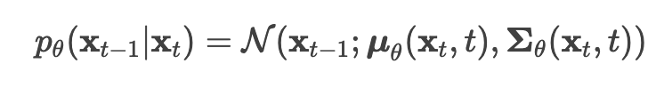
• μθ = neural network predicts the mean of reverse distribution
• Σθ = neural network predicts the variance (either fixed or not fixed, depending on βt)

The true conditional distribution q(xt-1|xt) is intractable, since it requires computing statistics of the true data distribution. So the solution is to approximate q(xt-1|xt) with a parameterized pθ(xt-1|xt) provided by a neural network. To summarize, both the forward and the reverse process: the forward process is pre-defined with sample images. A neural network is trained to predict the noise to reduct from pure noise until a clear sample image, where the time-dependent parameters of the Gaussian transitions are learned. Just like the forward process, formula for the full backward process can be found below with a summary of all formulas.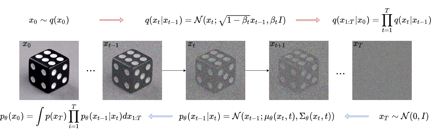

(source: Hugging Face blog: Diffusion Models) Given the length of this blog, we will be discussing more in detail about the reverse process, its link to training and more mathematical tachniques like ELBO and KL divergence.

Further down the road:

Now that we have built up an intuition towards the basic notion of how the diffusion process is carried out, we will proceed to other parts of diffusion models in the next blogs. In the next blogs we will dive deeper into understanding the details, and slowly gathering our building blocs.

Next from the series:

• DDPM training & loss
• U-net structure
• Stable diffusion part 1: latent space & VAE — veriational autoencoders
• Stable diffusion part 2: CLIP text encoder
• Intro into the Diffusers library
• On finetuning and LoRa
• … (more on the way)
  At the end, the order may be different from their releases and some contents may be added in between, but there will be more to come from the series.

Some sources I came across before writing this article, very useful if you like further readings:
GAN vs. Diffusion models
Hugging Face diffusion models overview
Medium article, How Stable Diffusion Works (with code example)
Fast.ai course chapter on Stable Diffusion:
Youtube video Diffusion Models Math Explained (if you are interested in the derivation of the formulas)
*Note: the citations in this blog are not put in a formal format, but the links are properly cited.